If a structural shock is not directly observable, neither can it be constructed through observable variables, we can identify it using an instrument variable approach if an instrument is available.
Suppose our observable space \(\boldsymbol y=(y_1,y_2,\dots)'\) is spanned by multiple structural shocks \(\epsilon = (\epsilon_1,\epsilon_2,\dots)'\). We want to identify the causal effect of structural shock \(\epsilon_1\). An instrument variable \(z\) satisfies the following conditions:
\(\mathbb E(\boldsymbol\epsilon_{t+j}z_t) = 0\) for \(j\neq 0\) (lead-lag exogeneity).
\(\epsilon_{2:n}\) denotes all other structural shocks except \(\epsilon_1\). The lead-lag exogeneity is unique to time series. To understand this, consider an local projection: \(y_{t+h} = \theta_h\epsilon_t +u_{t+h}\). As illustrated in the last section, \(u_{t+h}\) is a linear combination of the entire history of structural shocks. If \(z_t\) is to identify the causal effect of shock \(\epsilon_{1t}\) alone, it must be uncorrelated with all leads and lags. The requirement that \(z_t\) be uncorrelated with future \(\epsilon\)’s is generally not restrictive — by definition, future shocks are unanticipated. To the contrary, the requirement that \(z_t\) be uncorrelated with past \(\epsilon\)’s is more restrictive and hard to meet.
Suppose we want to estimate the causal effect of \(\epsilon_{1,t}\) on \(y_{2,t+h}\), where \(\epsilon_{1,t}\) is only observable through \(y_{1,t}\). Suppose we have an instrument variable \(z_t\) that satisfies the above conditions. The local projection
\[
y_{2,t+h} = \theta_{h,21} y_{1,t} + u_{t+h}
\]
cannot be consistently estimated because \(y_{1,t}\) and \(u_{t+h}\) are correlated. However, with the help with \(z_t\) as an instrument, we can consistently estimate the dynamic multiplier \(\theta_{h,21}\):
Lead-lag exogeneity implies \(z_t\) being unforecastable in a regression of \(z_t\) on lags of \(y_t\). If the exogeneity fails, LP-IV is not consistent. This problem can be partially addressed by including control variables in the regression:
We could also include lagged values of \(y_t\) or other lagged variables. The IV estimator is consistent if \(\boldsymbol w_t\) absorbs all past shocks that could potentially correlated with \(z_t\). In a broad sense, the validity of the instrument variable with additional controls requires that the controls span the space of all structural shocks.
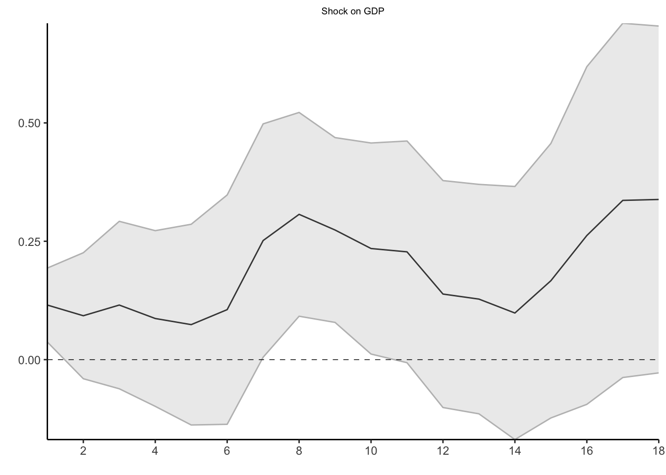
library(lpirfs)# Load dataag_data <-na.omit(ag_data)# Endogenous data (government spending, tax, GDP)endog <- ag_data[,3:5]# Variable to shock with (government spending)gov <- ag_data[,3]# Government spending shock identified by # Ramey and Zubairy (2018) using military newsgov_shock <- ag_data[,7]# Estimate linear model via 2SLSresults <-lp_lin_iv(endog, lags_endog_lin =4,shock = gov, instrum = gov_shock, use_twosls = T,trend =0, confint =1.96, hor =18)# Show all responsesplot_lin(results)[[3]]