Thus, \(\Phi_1=\rho+\zeta_1\), \(\Phi_s=\zeta_s-\zeta_{s-1}\), \(\Phi_p=-\zeta_{p-1}\). So the coefficients of the original VAR \(\{\Phi_s\}\) can be written as linearly combinations of coefficients on stationary regressors \(\{\zeta_s\}\). According to the theorem in Chapter 24, the asymptomatic distribution of \(\Phi_s\) would be dominated by slower converging \(\zeta_s\). It follows that \(\sqrt{T}(\hat\Phi_s-\Phi_s)\) is asymptotically Gaussian for \(s=1,2,\dots,p\). The usual OLS \(t\)-test and \(F\)-test are asymptotically valid. However, tests for Granger-causality based on VAR with unit roots do not have the usual \(\chi^2\) distribution, hence would not be valid.
32.1 Monte Carlo
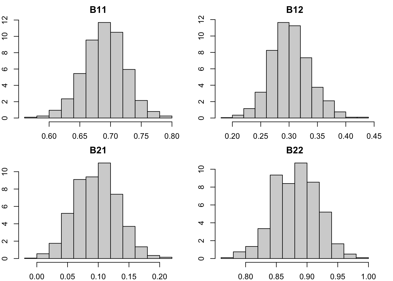
Below is a Monte Carlo simulation of a 2-dimensional VAR process with unit root, which verifies the Gaussian distribution of its coefficients.
library(tsDyn)library(vars)set.seed(0)bhat =sapply(1:1000, function(i) {# this is a VAR with unit root B =matrix(c(0.7, 0.1, 0.3, 0.9), 2)# simulate the VAR process sim <-VAR.sim(B, n =300, include ="none") mod =VAR(sim); b =coef(mod)# extract the coefficientsc(B11 = b$y1['y1.l1', 'Estimate'],B12 = b$y1['y2.l1', 'Estimate'],B21 = b$y2['y1.l1', 'Estimate'],B22 = b$y2['y2.l1', 'Estimate'])}) |>t()# plot the distribution of the coefficients{par(mfrow=c(2,2), mar=c(2,2,2,2))hist(bhat[,'B11'], freq=F, main="B11")hist(bhat[,'B12'], freq=F, main="B12")hist(bhat[,'B21'], freq=F, main="B21")hist(bhat[,'B22'], freq=F, main="B22")}
Distributions of the VAR coefficients by Monte Carlo simulation
32.2 Conclusions
Economic time series usually comes in seasonally-adjusted (log) levels, which often involve unit roots. Researchers have to make the choice whether to difference the data to stationary or leave it as it is when modelling. There is no single principle to rule them all. It depends on the purpose of the research. It might feel safe to work with stationary time series only. Though stationarity is not necessary for VARs to work properly. Here are the tips from Walter Enders:
To difference or not to difference
If the coefficient of interest can be written as a coefficient on a stationary variable, then a \(t\)-test is appropriate.
You can use \(t\)-tests or \(F\)-tests on the stationary variables.
You can perform a lag length test on any variable or any set of variables.
Generally, you cannot use Granger causality tests concerning the effects of a non-stationary variable.
The issue of differencing is important. If the VAR can be written entirely in first differences, hypothesis tests can be performed on any equation or any set of equations using \(t\)-tests or \(F\)-tests.
It is possible to write the VAR in first differences if the variables are \(I(1)\) and are not cointegrated. If the variables in question are cointegrated, the VAR cannot be written in first differences.