set.seed(1)

# generate two random walk processes
x = cumsum(rnorm(200))
y = cumsum(rnorm(200))

plot.ts(cbind(x,y), main="Two Random Walks")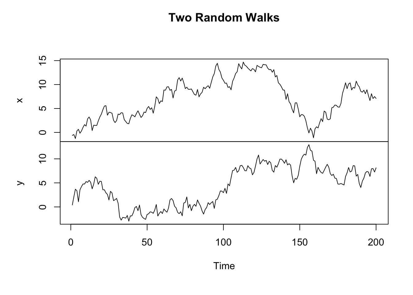
It is said, all stationary series are alike, but each non-stationary series is non-stationary in its own way (remember Leo Tolstoy’s famous quote: all happy families are alike; each unhappy family is unhappy in its own way.)
In all previous chapters, we have been working on stationary processes. We have shown that similar regression techniques and asymptotic results hold for stationary processes as for \(iid\) observations, albeit not exactly the same. If a time series is not stationary, we transform it to stationary by taking differences.
This chapter is devoted to study non-stationary time series. Special attention is given to unit root processes. We will see the theories involving non-stationary processes are entirely different from those applied to stationary processes. This makes unit root analysis an rather independent topic.
The obsession with unit root in academia have faded away in recent decades (I do not know if this assessment is accurate). Despite the topic posses immense theoretical interest, it does not seem to provide proportionate value for applied studies. Nonetheless, the topic is indispensable for a comprehensive understanding of time series analysis.
We start by pointing out that, it is very dangerous to blindly include non-stationary variables in a regression. To illustrate this, consider two random walks:
\[ \begin{aligned} x_{t} &= x_{t-1} + \epsilon_{t},\quad\epsilon_{t}\overset{iid}\sim N(0,\sigma_X^2)\\ y_{t} &= y_{t-1} + \eta_{t},\quad\eta_{t}\overset{iid}\sim N(0,\sigma_Y^2) \end{aligned} \]
\(\epsilon_t\) and \(\eta_t\) are independent to each other.
set.seed(1)
# generate two random walk processes
x = cumsum(rnorm(200))
y = cumsum(rnorm(200))
plot.ts(cbind(x,y), main="Two Random Walks")
We would expect the two series completely uncorrelated, as they are two independent random processes. However, if we regress \(y_t\) on \(x_t\), we would likely find a very strong correlation. This is called a spurious regression.
\[ y_t = \alpha + \beta x_t + u_t \]
lm(y ~ x) |> summary()
Call:
lm(formula = y ~ x)

Residuals:
   Min     1Q Median     3Q    Max
-6.831 -3.904  1.021  3.223  9.731

Coefficients:
            Estimate Std. Error t value Pr(>|t|)
(Intercept)  3.23975    0.56584   5.726 3.78e-08 ***
x            0.15324    0.06886   2.225   0.0272 *
---
Signif. codes:  0 '***' 0.001 '**' 0.01 '*' 0.05 '.' 0.1 ' ' 1

Residual standard error: 4.049 on 198 degrees of freedom
Multiple R-squared:  0.0244,    Adjusted R-squared:  0.01948
F-statistic: 4.953 on 1 and 198 DF,  p-value: 0.02718
Note that if we difference the two series to stationary, the spurious correlation disappears.
lm(diff(y) ~ diff(x)) |> summary()
Call:
lm(formula = diff(y) ~ diff(x))

Residuals:
     Min       1Q   Median       3Q      Max
-2.93078 -0.55055 -0.02841  0.67557  2.58926

Coefficients:
            Estimate Std. Error t value Pr(>|t|)
(Intercept)  0.03963    0.07203    0.55    0.583
diff(x)     -0.02171    0.07756   -0.28    0.780

Residual standard error: 1.015 on 197 degrees of freedom
Multiple R-squared:  0.0003974, Adjusted R-squared:  -0.004677
F-statistic: 0.07831 on 1 and 197 DF,  p-value: 0.7799
If we simulate many random walks, we would observe that a large percentage of the regressions report statistically significant relationships even though the series are independent.
# Simulation parameters
n <- 100         # Number of observations in each random walk
num_sim <- 1000  # Number of simulations
sig_count <- 0   # Counter for significant p-values
pvals <- numeric(num_sim)  # To store p-values

# Loop over simulations
for (i in 1:num_sim) {
  # Generate two independent random walks of length n
  x <- cumsum(rnorm(n))
  y <- cumsum(rnorm(n))

  # Run linear regression of y on x
  model <- lm(y ~ x)
  pval <- summary(model)$coefficients[2, 4]
  pvals[i] <- pval
}

# Calculate percentage of simulations with p-value < 0.05
sig_percent <- mean(pvals < 0.05) * 100
print(paste("Percentage of significant regressions:", sig_percent, "%"))
[1] "Percentage of significant regressions: 77 %"This example gives you a quantitative feel for how frequently spurious results can occur. What’s more interesting, however, is that we can eliminate this spurious strong correlation by including lags of dependent and independent variables —
# Compute lags for x and y
y_lag = dplyr::lag(y)
x_lag = dplyr::lag(x)

# Regression with lags
lm(y ~ y_lag + x + x_lag) |> summary()
Call:
lm(formula = y ~ y_lag + x + x_lag)

Residuals:
    Min      1Q  Median      3Q     Max
-2.6094 -0.6136  0.0433  0.7026  2.4059

Coefficients:
            Estimate Std. Error t value Pr(>|t|)
(Intercept)  0.34804    0.32558   1.069    0.288
y_lag        0.91403    0.03597  25.413   <2e-16 ***
x            0.12296    0.11279   1.090    0.278
x_lag       -0.05127    0.11040  -0.464    0.643
---
Signif. codes:  0 '***' 0.001 '**' 0.01 '*' 0.05 '.' 0.1 ' ' 1

Residual standard error: 1.076 on 95 degrees of freedom
  (1 observation deleted due to missingness)
Multiple R-squared:  0.9206,    Adjusted R-squared:  0.9181
F-statistic: 367.3 on 3 and 95 DF,  p-value: < 2.2e-16
Non-stationary time series can cause troubles, but they are also fascinating topics to explore. In what follows, we will focus on two types of non-stationary processes: trend-stationary processes and unit root processes, which are the most common types of non-stationary series we would encounter in economic and finance. Non-stationary series with exponential growth can be transformed into linear trend, hence is not of particular interest. We will start with the relatively easy tread-stationary processes, and spend most of the paragraphs on unit root processes.